Binned Fit — Least-Squares Fit and Binned Maximum-Likelihood Fit

2022-03-10

Prologue

This is a record of a workshop on statistics held among the High-Energy Physics group of National Taiwan University in 2022.

The textbook referred to throughout the record is Behnke, O. (2013) Data analysis in high energy physics a practical guide to statistical methods / edited by Olaf Behnke…[et al.]. 1st ed. Weinheim, Germany: Wiley-VCH.

In this week, we covered Sec.2.4–2.6, which was mainly about the method of least squares and maximum-likelihood fits.

The workshop was to let the participants reproduce the histogram fitting on $𝑀_{𝜇^{+} 𝜇^{-}}$ in Subsubsec.2.4.2.1.

ToolsIt’s assumed that you’ve already imported the familiar modules i.e. `import numpy as np; import matplotlib.pyplot as plt; import scipy.stats as st; import scipy.optimize as opt`.

`np.concatenate`

a = np.asarray([1, 2])
b = np.asarray([3, 4])
c = np.concatenate((a, b))  # Note the ntuple!
print(c)

[1 2 3 4]

`plt.hist`

Does not just draw a histogram, but also returns the histogram and the bins in use.

entries, bins, _ = plt.hist(st.norm.rvs(size=1000))

Least-Squares Fit

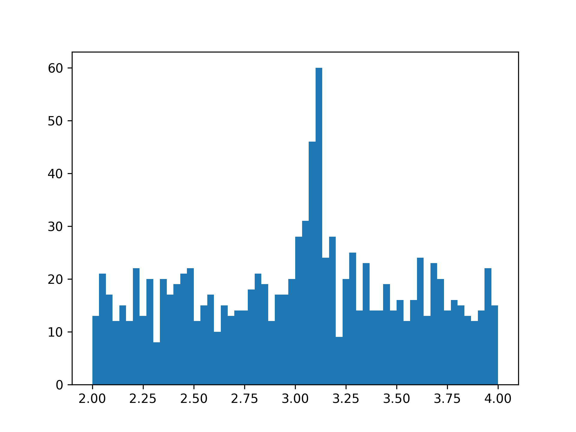
Prepare pseudo-data and histograms

By inspection and information given in the book, it seems that

the number of bins is 60,
the background events can be simulated by st.uniform(loc=2, scale=2) and the event number is roughly 1000, and
the signal events can be simulated by st.norm(loc=3.1, scale=0.05) and the event number is roughly 100.

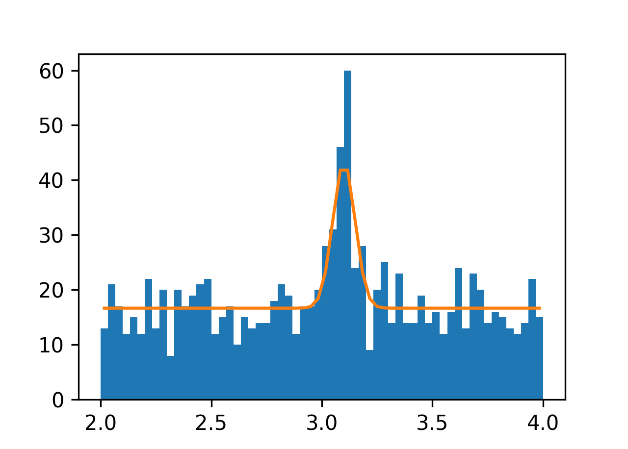
Construct expected number of events in each bin

Assuming we know the exact numbers of background and signal events, then the number of events in each bin is just

𝑓_{𝑖} = 1000 \cdot 𝑓_{𝑖}^{𝐵} + 100 \cdot 𝑓_{𝑖}^{𝑆},

where $𝑓_{𝑖}^{𝐵}$ and $𝑓_{𝑖}^{𝑆}$ are probabilities of events in the $𝑖$ -th bin i.e.

\begin{aligned} 𝑓_{𝑖}^{𝐵} & = \int_{𝑥_{𝑖}^{l o w}}^{𝑥_{𝑖}^{u p}} 𝑓^{𝐵} (𝑥) 𝑑 𝑥, \\ 𝑓_{𝑖}^{𝑆} & = \int_{𝑥_{𝑖}^{l o w}}^{𝑥_{𝑖}^{u p}} 𝑓^{𝑆} (𝑥; 𝑀) 𝑑 𝑥 . \end{aligned}

In the discrete case, we can approximate the integral as

𝑓_{𝑖}^{𝐵} = \int_{𝑥_{𝑖}^{l o w}}^{𝑥_{𝑖}^{u p}} 𝑓^{𝐵} 𝑑 𝑥 \approx \sum_{𝑖} 𝑓^{𝐵} (𝑥_{𝑖}^{𝑐}) Δ 𝑥_{𝑖},

and so on, where $𝑥_{𝑖}^{𝑐}$ is the center of the bin i.e. $𝑥_{𝑖}^{𝑐} = (𝑥_{𝑖}^{u p} + 𝑥_{𝑖}^{l o w}) / 2 .$

The expected number of events, when drawn on the previous plot, should look like this. Here M = 3.1. — The expected number of events, when drawn on the previous plot, should look like this. Here $𝑀 = 3.1$ .

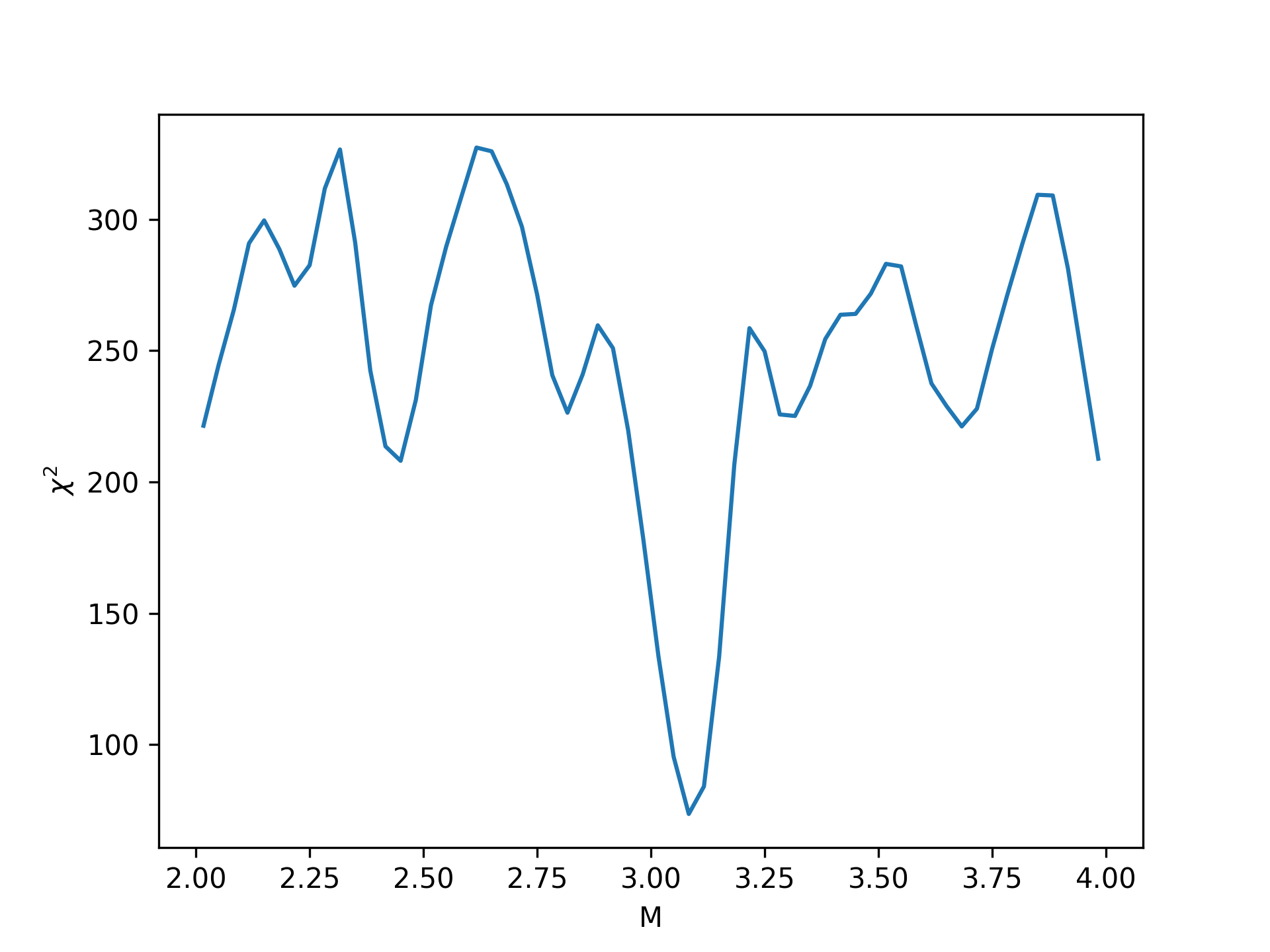
Calculate, plot and minimize $𝜒^{2}$

Recall that the (Neyman’s) $𝜒^{2}$ value can be calculated as

𝜒^{2} (𝑀) = \sum_{bin 𝑖} \frac{{[𝑘_{𝑖} - 𝑓_{𝑖} (𝑀)]}^{2}}{𝑘_{𝑖}} .

Your \chi^2 values should look like this. — Your $𝜒^{2}$ values should look like this.

Binned Maximum-Likelihood Fits

Use the same dataset (and the same histogram) to perform Binned MLE. Note that the log-likelihood in the binned case is

ln 𝐿 (𝑀) = \sum_{𝑖 = 1}^{𝐵} 𝑘_{𝑖} ln 𝑃_{𝑖} (𝑀) + constant,

where $𝑃_{𝑖} (𝑀)$ is the likelihood computed with the probability of events falling within the $𝑖$ -th bin.

Remarks

On Numbers of Generated Events

What would happen if we only generated st.norm.rvs(loc=3.1, scale=0.05, size=100) and set bins as np.linspace(-5, 5, 101) instead? What assumption of Least-Squares Fit would be violated? What Python error would you get?

On Assumptions of Event Numbers

Recall that we assume that we know the exact numbers of both signal and background events. That is not a common situation in practice, though. We typically need to turn those event numbers into parameters as well. And that is what the next week’s workshop is about, Extended Maximum-Likelihood Fits.

On $𝜒_{min}^{2}$

You may get $𝜒_{min}^{2}$ deviated from the expected value, which is 59, as much as, say, 68. Do you think it’s reasonable? (Hint: go the wikipedia page of $𝜒^{2}$ distribution and look for the quantity related to expected deviation from the expected value.)